Finding Seasonal Spreads

Paul Teetor

Many spreads show seasonality -- that is, regular patterns from year-to-year -- and can be a valuable source of profits and diversification. Seasonal spreads, however, seem to get little attention from the quantitative community. I’d like to remedy that by showing one way to identify seasonal spreads using legitimate statistical techniques. I'll start with an example of a seasonal spread: crude oil versus gasoline.

Example: Crude oil versus gasoline

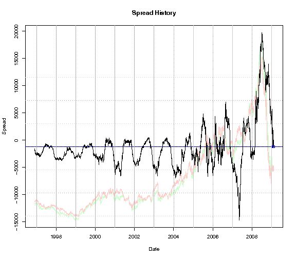
Here is a chart of the spread between crude oil futures (CL) and gasoline futures (RB) from 1997 to the present, covering about 12 years of history.

If you look closely, it appears that the spread often falls during Winter, then rises from Spring into Summer. But how can we be sure? Perhaps we are just imagining the pattern, based on a few examples. And what are the actual months when it falls and rises?

Here is how we can test for a seasonal pattern.

Compute the daily change in the spread, s_t, giving us one Δs_t value for every day of the spread’s history.
For each day, group the day’s change according to the month of that day.
Compute the average change for each monthly group.

That will give a table such as this, with one mean change (µ) for every month, taken over all the years of spread history.

	Jan	Feb	Mar	Apr	May	Jun	Jul	Aug	Sep	Oct	Nov	Dec
Mean change	-31.97	52.15	-16.74	12.98	94.73	78.16	33.08	-12.39	-18.88	22.77	-121.50	-90.37

(These averages are in dollars per day.)

The monthly averages suggest trades: January is a down month, on average, so sell the spread during January. Likewise, February is an up month, on average, so buy the spread during February.

Those trades would be very naïve, however. A statistician would ask an important question before risking real money: What is probability that the true mean is actually positive or negative? The averages for April and August are pretty small (12.98 and -12.9), for example. Maybe our sample is too small, and these averages are not representative. How realistic are these numbers?

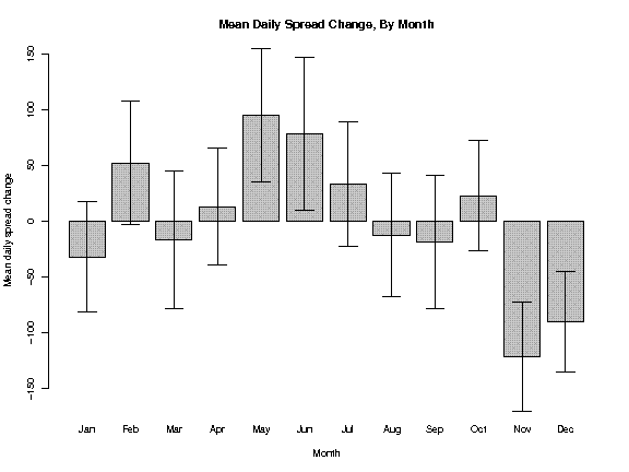
The solution is to form confidence intervals for each monthly mean. This barchart shows the mean change taken from the table above, then superimposes the confidence intervals over each bar, giving us a composite view of the monthly averages.

Barchart of mean daily spread change by month

Consider the bar for January. Yes, the mean change is negative, but the confidence interval crosses over into positive territory. Statistically speaking, we cannot be confident that the true mean is negative. It could be zero or even positive, so selling the spread during January could be unwise. In fact, the confidence interval includes zero for most months, and we cannot be confident there is any seasonal trend in those months, either positive or negative.

The confidence interval for May, however, is completely positive. We can be confident that the average historical daily change in May is positive. In fact, May and June are clearly “up” months, and November and December are clearly “down” months. Now we have our seasonal trade for the CL/RB spread:

Buy the spread on May 1. Close the position on Jul 1.
Short the spread on Nov 1. Close the position on Jan 1.

Finding Seasonal Spreads Automatically: ANOVA

This analysis would be quite tedious if we performed it manually for every spread we know. Fortunately, we can use ANOVA to automatically identify seasonality in spreads.

ANOVA stands for analysis of variance. ANOVA compares groups of observations, such as our month-wise groups of spread changes. It reports the probability that one or more groups have significantly different means, compared with the other groups.

The ANOVA report includes a probability value, or simply p-value, which is the probability that all the means are identical. So a small p-value means one or more groups are probably not the same. In the CL/RB example, above, my computer reports a p-value of less than 0.0001, so the probability that all months have the same average change is less than 0.01%.

My computer runs a weekly batch job which computes the ANOVA p-value for every spread in my database. If the p-value is 0.05 or less, I know there is a 95% probability that the spread changes are significantly different from month-to-month; in other words, the spread exhibits a seasonal pattern. In those cases, the batch job saves the p-value in the database. Later, I run a report to select the spreads with the best (i.e., smallest) p-values. Those are my candidates for seasonal trades.

The computer tests every combination of stocks and futures, so it occasionally reports a bizarre seasonal spread. It recently discovered that the spread between British Pound futures (BP) and Live Cattle (LC) shows seasonality at a confidence level of 96% or better. Would I trade the BP/LC spread? Of course not, because I cannot discern the economic logic of the trade.

Limitations

This analysis is not an automated trading system and has important limitations.

The analysis does not make a prediction. It only reports the past pattern. When you trade that pattern, you are assuming this year is like other years.
The basic ANOVA analysis only reports that some months are different, not which months are different. The trader must look at monthly pattern to choose the right time for the trade.
The trade decision must also incorporate the current market conditions. For example, if the history recommends buying but the spread is already quite high, the trade could be unwise.
This analysis looks at monthly patterns. The seasonal patterns at other boundaries might be more distinct and, hence, better trades.

Next Steps

We can augment this analysis by computing the spread’s Z score, then selecting trades which show harmony between their historical pattern and current status. We can also improve the analysis by incorporating a seasonal version of the Ornstein-Uhlenbeck formula, letting us predict the time-to-profit. I hope to cover these subjects in the future.

Additional Details For the Curious

The data for the CL/RB spread, above, was purchased from Commodity Systems Inc. (CSI), using their Perpetual Contact data. This example was as of Feb 5, 2009.

When I say “long the CL/RB spread”, I mean buy CL and sell RB. Likewise, “short the spread” means sell CL and buy RB.

I compute the hedge ratios for my spreads using ordinary least squares, as suggested in Ernie Chan's book. The ratio for the CL/RB spread, above, was 1.1376 CL contracts for each RB contract.

Notice that I compute the spread change, not the spread return. Quants usually study price returns, but that won’t work with spreads because the spread can be zero, giving an undefined return. The daily change follows a similar bell-shaped distribution, so it’s a reasonable object for study.

I monitor about 115 stocks and futures, so I have about 6,670 spreads to be tested weekly. A typical recent run found that over 270 spreads that exhibit some seasonality, or about 4% of those tested. The ANOVA batch job requires about 2-1/2 hours to complete on my computer. The software is written in a combination of Perl and R, the free statistical software system, running under Linux.

References

The original and still-the-best book on seasonality is Seasonality: Systems, Strategies, and Signals, by Jake Bernstein. Some of the ideas in this analysis were inspired by Bernstein’s book.

Most good textbooks on statistics discuss ANOVA. There is an article on Wikipedia, but it is not a tutorial.

Any decent software for statistics includes the ANOVA analysis. That includes R and Octave, which are both free.